library(dplyr)
library(ggplot2)
library(tidyr)
library(forcats)
library(purrr)
library(nmmr)
library(glue)

size_shape <- 2
set.seed(1234)

How can neuromodulation be assessed quickly?

A key insight of NMM is that, under certain circumstances, neuromodulation is reflected in changes to the voxel tuning function. That is, changes in the voxels tuning function implicate certain forms of neuromodulation. NMM outlines two techniques for looking at voxel tuning functions. One technique, a Bayesian modeling approach, requires assuming that the neural tuning functions and distributions of neurons within voxels follow a specific form. The Bayesian component of NMM pools information across voxels with hierarchical modeling, boiling down the question of neuromodulation into model comparison. But the Bayesian model assumes that the weight distribution and neural tuning function follow specific functional forms, assumptions that may not hold in all datasets (e.g., with some voxel sizes, the weight distribution may be multimodal). Moreover, the full Bayesian model is complex, making it challenging to assess which features of the data drive a comparison in favor of multiplicative gain versus additive offset. So, the Bayesian approach makes assumptions that may not always hold, is computationally expensive, and is hard to understand.

To complement the parametric modeling, NMM includes a non-parametric method for checking the form of neuromodulation, covered in this vignette.

Non-parametric Check

Ideally, we could assess changes in the voxel tuning functions by simply plotting them. Generating that plot is easy enough. This package comes with the dataset sub02, which contains the responses for voxels in V1 for a single participant (author PS). Here are the tuning functions for six of those voxels.


# take six voxels worth of data and calculate summary statistics
six_voxels <- sub02 %>%
  group_by(contrast, orientation, run, ses) %>%
  slice_head(n = 6) %>%
  group_by(voxel) %>%
  group_nest() %>%
  mutate(
    data = map(
      data, 
      ~WISEsummary(.x, dependentvars = y, withinvars = c(orientation, contrast)))) %>%
  unnest(data)

# plot the tuning functions
six_voxels %>%
  ggplot(aes(x=orientation, y=y_mean, color = contrast)) +
  facet_wrap(~voxel, labeller = label_both) +
  geom_line() +
  geom_errorbar(aes(ymin=y_mean-y_sem, ymax=y_mean+y_sem)) +
  ylab("Average BOLD Signal (% Average Signal)")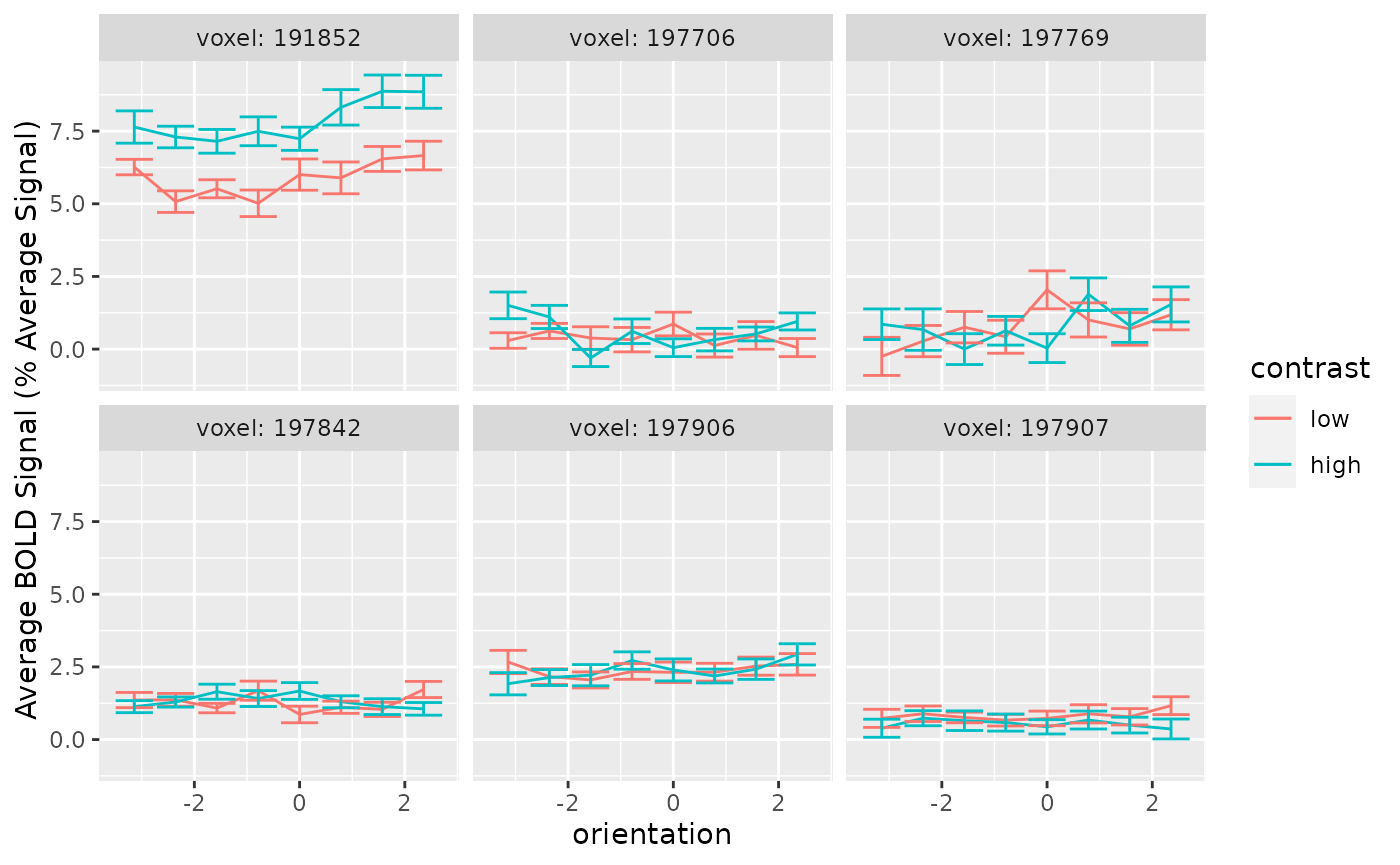

Individual voxel tuning functions are too noisy to provide information about neuromodulation individually. Error bars span 95% confidence intervals

Although intuitive, plots of the voxel tuning function are uninformative. This is because most voxels have weak tuning. That is, across orientations, the lines are nearly flat, and the activity is rather variable. When tuning is weak, different forms of neuromodulation look identical (i.e., multiplying a flat line by a gain factor can produce the same result as simply adding an offset). So, simply plotting the voxel tuning functions does not offer much insight into the form of neuromodulation.

A scatter plot of activity across conditions reveals changes in voxel tuning

The central idea, detailed in the main paper, is that we can assess multiplicative vs. additive shift by looking at the slope of a line made from the low-contrast activity plotted against the high-contrast activity. That is, a key difference between the models we compared is that the multiplicative model allows the effect of contrast to vary by orientation whereas the additive model does not. Additive neuromodulation corresponds to an increase in neural activity at all orientations. Thus, regardless of the forms of the weight distribution and neural tuning function, additive neuromodulation causes the low-contrast tuning function to shift upwards uniformly across orientations. Hence, a scatter plot of the voxel’s response to high-contrast stimuli against its response to low-contrast stimuli has a slope of 1. In contrast, multiplicative neuromodulation corresponds to an increase in neural activity at the most preferred orientations, and a scatter plot of a voxel’s response to high versus low-contrast stimuli has a slope larger than 1. Therefore, the models can be differentiated by plotting high-contrast activity against low-contrast activity and calculating the slope of the best fitting line. A slope of one implies additive shift, but a slope greater than one implies multiplicative gain.

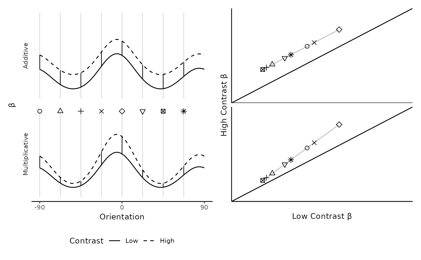
Plotting beta a voxel’s response to high- versus low-contrast uncovers neuromodulation. Left: Simulated voxel tuning functions in which higher levels of contrast induce either an additive (top) or multiplicative (bottom) neuromodulation. The eight vertical lines are eight hypothetical orientations at which these voxel tuning functions might be probed, which would produce eight responses per level of contrast. Right: The two kinds of neuromodulation reveal different signatures when the response to high-contrast stimuli are plotted against the response to low-contrast stimuli. The diagonal line corresponds to no effect of contrast. A line drawn through the points produced by the additive model necessarily has a slope equal to 1; under this neuromodulation, the effect of contrast does not depend on the orientation. A line drawn through the points produced by the multiplicative model necessarily has a slope greater than 1; under this neuromodulation, the effect of contrast is largest at those orientations which are closest to the voxel’s preferred orientation.

Orthogonal Regression

Based on the above, we know that different forms of neuromodulation are implicated by the slope of a line fit to high- versus low-contrast activity. However, to estimate this line, we should not estimate the line with ordinary least squares. This subsection will overview why ordinary least squares is insufficient, suggesting instead orthogonal regression orthogonal regression.

Sample Data

Here is a toy example to build intuition for the failings of ordinary least squares as an estimate of slope in this situation. Let the variable \(z\) refer to the average activity of a voxel at low contrast. For simplicity, assume that this variable is distributed according to a standard normal distribution.

\[ z \sim N(0, 1) \]

As researchers, we are unable to directly observe \(z\); this variable is the average activity at low contrast, but on any given trial a voxel’s response varies around the average. Assume that the variability follows another standard normal distribution, so the resulting observed activity at low contrast, \(x\), is distributed according to another normal distribution

\[ x \sim N(z, 1) \]

The activity at high contrast will be a function of the activity at high contrast. In this toy example, let’s assume multiplicative gain factor of two. Importantly, the activity at high contrast will be a function of the latent voxel tuning function, \(z\), not the noise-corrupted observation, \(x\). Activity at high contrast, \(y\), will then be distributed according to the following (again, assuming standard normal noise).

\[ y \sim N(2z, 1) \]

Together, these assumptions define a model from which we can simulate datasets. The following chunk defines a function for simulating from this toy model and then uses it to generate 1000 observations (i.e., this would be 1000 observations for a single voxel at each of low and high contrast).

simulate_toy <- function(N, true_slope = 2){
  tibble(z = rnorm(N)) %>%
    mutate(
      x = rnorm(N, z),
      y = rnorm(N, 2*z))
}

d <- simulate_toy(N = 1000)

Ordinary Least Squares will not work

We can use the built-in function lm to estimate the slope with ordinary least squares.

ls <- lm(y ~ x, data=d)
ls
#> 
#> Call:
#> lm(formula = y ~ x, data = d)
#> 
#> Coefficients:
#> (Intercept)            x  
#>    -0.01208      1.00627

At only about 1.01, the estimated slope is only about half of the true slope (2)! The following plot shows the difference between the line we wanted to estimate (with a slope of 2), versus the line provided by lm.

d %>%
  ggplot(aes(x=x, y=y)) +
  geom_point(alpha = .2) +
  geom_abline(intercept=coef(ls)[1], slope=coef(ls)[2], color="blue") +
  coord_fixed() +
  ggtitle(glue("OLS slope: {round(coef(ls)[2], digits=2)}")) +
  geom_abline(intercept=0, slope=2, linetype = "dashed", color="blue")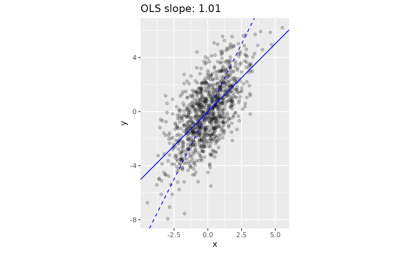

We want to estimate the dashed line, which has a slope of 2. However, Ordinary Least Squares (OLS) provides an estimate that is biased towards 0 (solid line).

This issue is known as Regression Dilution. One way to understand the issue that that there is variability in, not just the y-coordinate, but also the x-coordinate, which inspires the name errors-in-variables model ¹. For these circumstances, we need to use a orthogonal regression.

Orthogonal regression accurately recovers our desired slope

The nmmr package provides a function to estimate the slope, called get_slope. It takes two vectors of numbers. Here is how to apply it on our toy example

slope <- get_slope(d$x, d$y)
slope
#> [1] 1.952462

This is much closer to the true slope!

But perhaps we got lucky. Let’s stimulate 1000 datasets, estimating for each the slope with both ordinary least squares and orthogonal regression.

fits <- crossing(i = 1:1000) %>%
  mutate(simulation = map(i, simulate_toy, N=1000)) %>%
  rowwise() %>%
  mutate(
  ordinary = lm(y ~ x, data=simulation) %>% coef() %>% magrittr::extract(2),
  orthogonal = get_slope(simulation$x, simulation$y)) %>%
  select(-simulation) %>%
  pivot_longer(c(ordinary, orthogonal), names_to = "Method", values_to = "Estimate")

Next, plot the distribution of recovered slopes for each of the two methods.

fits %>%
  ggplot(aes(x=Estimate)) +
  geom_histogram(aes(fill=Method), bins = 100) +
  geom_vline(xintercept = 2, linetype = "dashed")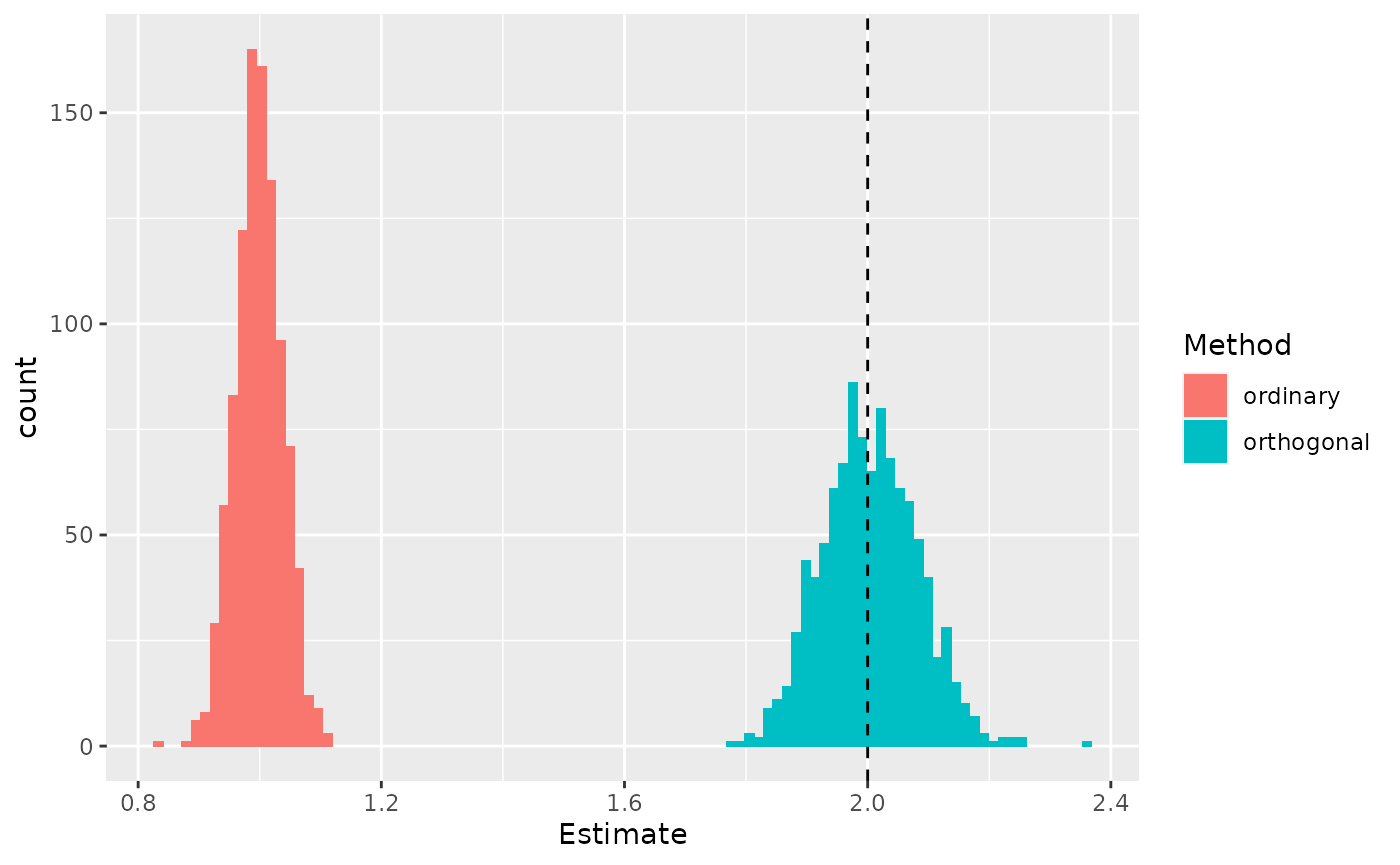

Across many simulated datasets, the ordinary least squares method estimates a slope that is too small, whereas the orthogonal regression is unbiased. The dashed vertical line marks the true slope.

These simulations suggest that ordinary least squares is indeed biased, whereas orthogonal regression gives a more accurate slope.

Application to data

We can apply this same method to estimate a slope for each voxel in the provided dataset, sub02. To use get_slope, first widen the data.

sub02_wide <- sub02 %>%
  pivot_wider(names_from = contrast, values_from = y)

sub02_wide
#> # A tibble: 26,928 x 7
#>    sub   run   voxel  orientation ses      low    high
#>    <fct> <fct> <fct>        <dbl> <fct>  <dbl>   <dbl>
#>  1 2     15    191852       0.785 3      3.36   6.39  
#>  2 2     15    197706       0.785 3     -2.84   0.0160
#>  3 2     15    197769       0.785 3     -2.03   4.14  
#>  4 2     15    197842       0.785 3      2.23   2.35  
#>  5 2     15    197906       0.785 3      2.86   2.11  
#>  6 2     15    197907       0.785 3      1.51   0.504 
#>  7 2     15    203688       0.785 3     -2.75   0.241 
#>  8 2     15    203689       0.785 3     -2.51  -2.34  
#>  9 2     15    203690       0.785 3     -3.16  -1.40  
#> 10 2     15    203753       0.785 3      0.711  0.427 
#> # … with 26,918 more rows

As mentioned above, contrast seems to have a different effect on each voxel. Hence, we should calculate the slope for each voxel separately. The nmmr package provides a helper function for applying the get_slope function to groups of a dataset, called get_slope_by_group.

slopes <- sub02_wide %>%
  get_slope_by_group(voxel, low, high)

For visualization, plot the distribution of estimated slopes.


slopes %>%
  ggplot(aes(x=slope)) +
  geom_histogram(bins = 200)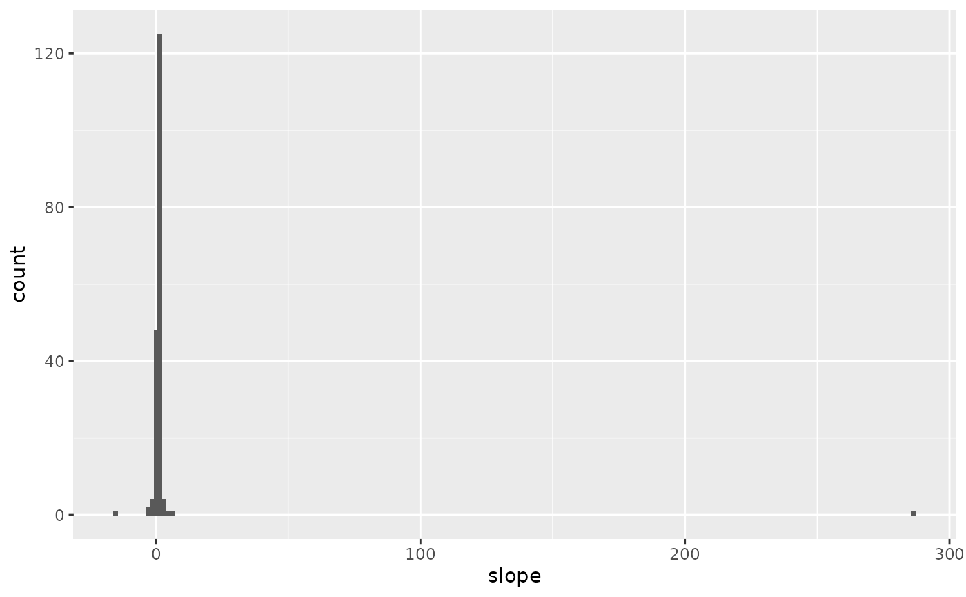

When looking at all of the voxels, some of the slopes are spuriously high.

Unfortunately, this distribution of slopes is not helpful. Clearly, there are outliers (e.g., one voxel has a slope that is over 200). These outliers are symptomatic of two challenges identified at the beginning of this voxel: voxels are flat and noisy. We can see the issue by looking at the activity for a single voxel.

sub02_wide %>%
  filter(fct_match(voxel, "209671")) %>%
  ggplot(aes(x=low, y = high)) +
  geom_point() +
  coord_fixed()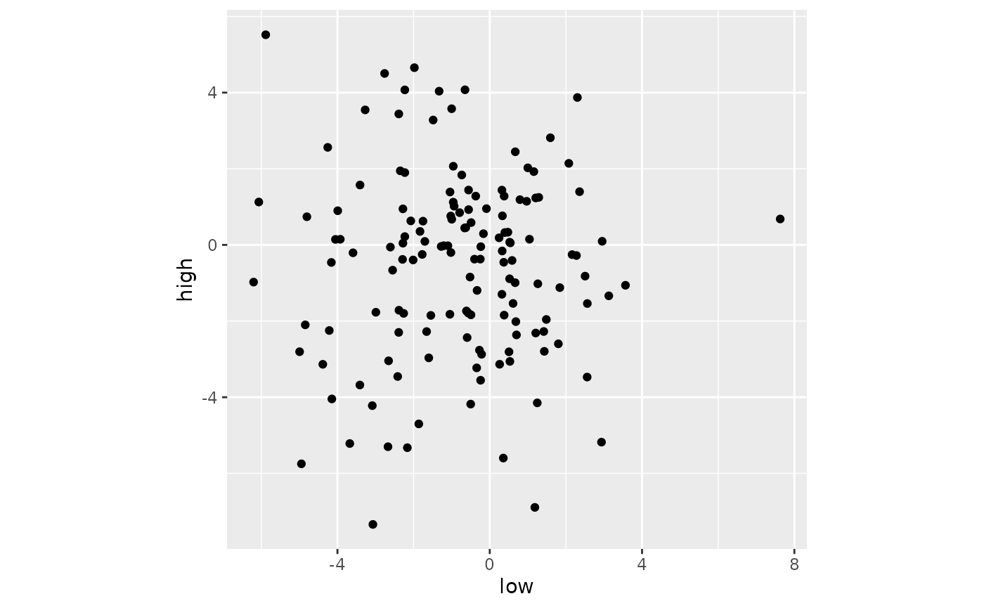

When voxels are poorly tuned, the best-fitting line can easily be one that is nearly vertical.

When a voxel is tuned weakly, the scatter plot is nearly circular. When the data are circular, a line at any angle fits equally well. So, with circular scatter plots, orthogonal regression often produces slopes that have a spuriously high slope.

Thresholding

Orthogonal least squares allows us to focus on the form of neuromodulation, but now we need a way to focus on just those voxels that are responsive to stimulation. In the paper, we advise thresholding based on each voxel’s responsivity to contrast. That is, we advise considering each voxel’s average difference in activity between high and low contrast, and then selecting only those voxels whose differences are in the upper quantiles.

sub02_wide %>%
  mutate(diff = high - low) %>%
  group_by(voxel) %>%
  summarise(average_difference = mean(diff)) %>%
  ggplot() +
  geom_histogram(
    aes(x=average_difference),
    bins = 20)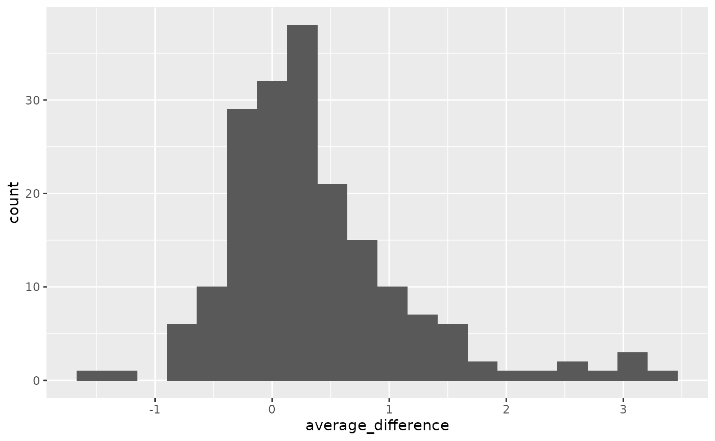

Distribution of average difference between high and low contrast, across voxels. The thresholding is based on the quantiles of this distribution.

In the paper, we looked at quatiles of 0 (i.e., no thresholding, analyze all voxels), and 0.9 (i.e., select only the top 10% of voxels within a participant). The nmmr function cross_threshold takes a dataframe and a vector of quantiles, and it returns another dataframe that can be used to filter voxels in the original data.

ranks <- cross_threshold(sub02_wide, voxel, low, high, quantiles = c(0, 0.9))

Joining the returned dataframe with the original dataset allows us to plot the distribution of slopes at both thresholds.

left_join(ranks, slopes, by = c("voxel")) %>%
  ggplot(aes(x=slope)) +
  facet_wrap(~Threshold, scales = "free", labeller = label_both) +
  geom_histogram(bins = 20) +
  geom_vline(xintercept = 1)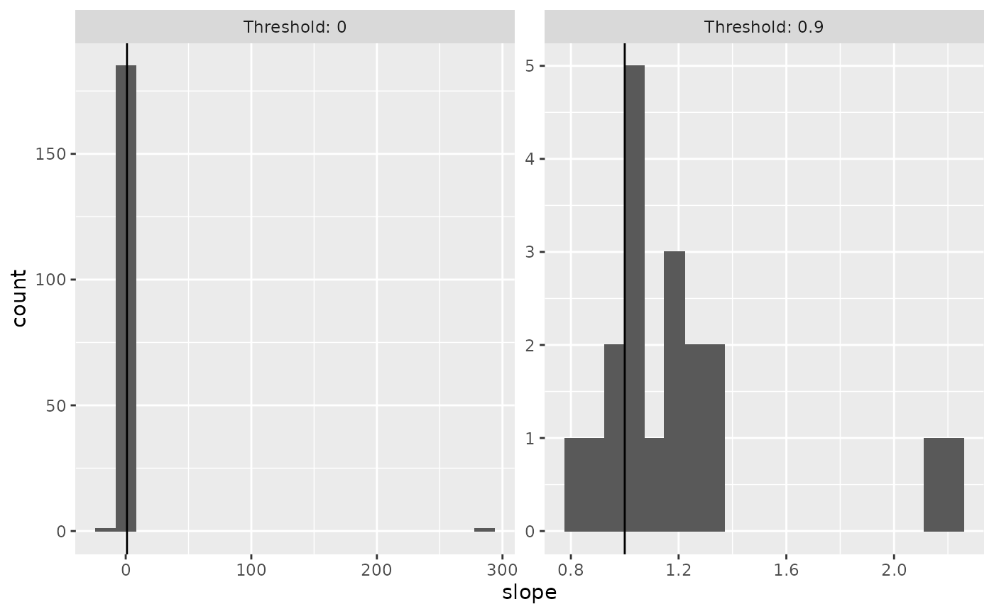

Thresholding based on the average difference across levels of contrast removed the spuriously high slopes. Vertical line marks a slope of 1, which is predicted by the additive but not multiplicative model.

This need to threshold is ad hoc; there is no clear reason why we should look at the top 10% of voxels, rather than the top 20% or 5%. But the point of this orthogonal regression is not to produce a precise measure of neuromodulation. Instead, it is meant as a rough-and-ready tool for checking whether neuromodulation is additive or multiplicative. In the nmmr package, the main functions for performing these checks are get_slope, get_slope_by_group, and cross_threshold.

If you need a method that is more quantitative, nmmr provides two other sets of functions, each covered in their own vignette. The most complex is the full Bayesian model. As outlined above, the Bayesian method uses hierarchical modeling to pool information across voxels. However, it also makes assumptions that may not hold in all datasets. For this reason, nmmr includes an intermediate approach, which implements the orthogonal regression idea in a Bayesian hierarchical model This has the advantage of still being quick (relative to the main Bayesian approach), but does not require ad hoc thresholding.

The intermediate approach is covered in vignette("deming-regression")

Put another way, ordinary least squares assumes a model like \(y \sim N(2x, 1)\) – e.g., that the activity at high contrast is directly related to the activity at low contrast↩︎