library(nmmr)
library(tidyr)
library(ggplot2)
library(dplyr)
#> 
#> Attaching package: 'dplyr'
#> The following objects are masked from 'package:stats':
#> 
#>     filter, lag
#> The following objects are masked from 'package:base':
#> 
#>     intersect, setdiff, setequal, union
library(forcats)

set.seed(1234)

Introduction

The vignette("orthogonal") presented a quick, non-parametric approach for checking neuromodulation based on a scatter plot of voxel activity at high- versus low-contrast. However, that method required an ad hoc preprocessing step, excluding poorly tuned voxels. Without this preprocessing, the estimated slopes were too variable. To obviate the need for filtering voxels, this vignette covers another set of functions that implement the scatter plot idea in a Bayesian hierarchical framework.

Bayesian Hierarchical Deming Regression

The Model

The model is very similar to the model underlying orthogonal regression, but for two important changes. First, the model is hierarchical. That is, whereas we previously ran a separate orthogonal regression on each voxel, we now estimate each of the separate slope, intercept, and noise terms in a single regression model¹. Second, we relax the assumption that the variances in both observed variables (e.g., voxel activity at high and low contrast) are equal².

The paper has full details of the model, but a plate diagram for the model is is reproduced here.

$Schematic of the Bayesian model. Filled square nodes indicate priors, open circles are estimated parameters, the shaded circles are observed data, and the open diamond is the result of a deterministic function of the parameters. Nodes are grouped with the square "plates", indicating over which subsets of the data the node is replicated. The distribution assigned to each node is listed to the right of the diagram. $N(\mu,\sigma)$ is a normal with location $\mu$ and scale $\sigma$, and $TN(\mu,\sigma)$ is a normal with the same parameters, truncated below at $\mu$. Each equation in the upper right is associated with an arrow in the diagram, describing a relationship between nodes.$

Schematic of the Bayesian model. Filled square nodes indicate priors, open circles are estimated parameters, the shaded circles are observed data, and the open diamond is the result of a deterministic function of the parameters. Nodes are grouped with the square “plates”, indicating over which subsets of the data the node is replicated. The distribution assigned to each node is listed to the right of the diagram. $N(\mu,\sigma)$ is a normal with location $\mu$ and scale $\sigma$, and $TN(\mu,\sigma)$ is a normal with the same parameters, truncated below at $\mu$. Each equation in the upper right is associated with an arrow in the diagram, describing a relationship between nodes.

Application to data

Data Prep

As for the orthogonal regression functions, the data need to be in a wider format. Additionally, the tuning variable (e.g., orientation) should be converted into a factor.

sub02_wide <- sub02 %>%
  pivot_wider(names_from = contrast, values_from = y) %>%
  mutate(orientation = factor(orientation))

For the purposes of this vignette, we reduce the dataset down to just 100 voxels. This is only to speed up the estimation process.

small <- sub02_wide %>%
  group_by(orientation, run, ses) %>%
  slice_head(n = 10) %>%
  mutate(voxel = fct_drop(voxel)) %>%
  ungroup()

Stan Code

The model can be implemented by initializing an object provided by the nmmr package of class Deming, using the $new() method. This method takes a dataset and the names of the columns with the two dependent variables (e.g., low and high). Additionally, the class needs to know which column contains the tuning variable (e.g., orientation) and the column indexing voxel (e.g., voxel).

m <- Deming$new(small, low, high, tuning_var = orientation, voxel_var = voxel)

The newly created object, m, is an R6 object of class Deming. It can be thought of as a wrapper around an instance of a cmdstanr::CmdStanModel class, but one which prepares the data for sampling. The actual model is contained in a field of m called cmdstanmodel. The underlying Stan model can be accessed with the $print() method of the cmdstanmodel field.³

m$cmdstanmodel
#> data {
#>   int<lower=1> n;  // total number of observations
#>   int n_voxel;
#>   int<lower=1, upper=n_voxel> voxel[n];
#>   int n_tuning;
#>   int<lower=1, upper=n_tuning> tuning[n];
#>   int<lower=1, upper=n_tuning*n_voxel> voxel_tuning[n]; // index to pick out from matrix of tuning x voxel
#>   vector[n] y;  // response variable (high)
#>   vector[n] x;  // noisy values (low)
#> 
#>   // priors
#>   vector[2] prior_z_mu_mu;
#>   vector[2] prior_z_mu_sigma;
#>   vector[2] prior_z_sigma_mu;
#>   vector[2] prior_z_sigma_sigma;
#>   vector[2] prior_x_sigma_mu;
#>   vector[2] prior_x_sigma_sigma;
#>   vector[2] prior_y_sigma_mu;
#>   vector[2] prior_y_sigma_sigma;
#>   vector[2] prior_g_mu;
#>   vector[2] prior_g_sigma;
#>   vector[2] prior_a_mu;
#>   vector[2] prior_a_sigma;
#> }
#> parameters {
#>   real<lower=0> g_sigma;
#>   real g_mu;
#>   vector<multiplier=g_sigma, offset=g_mu>[n_voxel] g;
#>   real<lower=0> a_sigma;
#>   real a_mu;
#>   vector<multiplier=a_sigma, offset=a_mu>[n_voxel] a;
#>   real<lower=0> z_mu_sigma;
#>   real z_mu_mu;
#>   row_vector[n_voxel] z_mu;
#>   matrix[n_tuning, n_voxel] z_raw;
#>   real<lower=0> z_sigma_sigma;
#>   real<lower=0> z_sigma_mu;
#>   vector<lower=-z_sigma_mu/z_sigma_sigma>[n_voxel] z_sigma_raw;
#>   real<lower=0> x_sigma_sigma;
#>   real<lower=0> x_sigma_mu;
#>   vector<lower=0>[n_voxel] x_sigma;
#>   real<lower=0> y_sigma_sigma;
#>   real<lower=0> y_sigma_mu;
#>   vector<lower=0>[n_voxel] y_sigma;
#> }
#> transformed parameters{
#>   vector[n_tuning*n_voxel] zeta;
#> 
#>   {
#>     matrix[n_tuning, n_voxel] z;
#>     vector[n_voxel] z_sigma = z_sigma_mu + z_sigma_raw * z_sigma_sigma;
#>     for (v in 1:n_voxel) z[,v] = z_sigma[v] * z_raw[,v] + z_mu[v];
#>     zeta = to_vector(z);
#>   }
#> 
#> }
#> model {
#>   z_mu_mu ~ normal(prior_z_mu_mu[1], prior_z_mu_mu[2]);
#>   z_mu_sigma ~ normal(prior_z_mu_sigma[1], prior_z_mu_sigma[2]);
#>   z_mu ~ normal(z_mu_mu, z_mu_sigma);
#> 
#>   to_vector(z_raw) ~ std_normal();
#> 
#>   z_sigma_mu ~ normal(prior_z_sigma_mu[1], prior_z_sigma_mu[2]);
#>   z_sigma_sigma ~ normal(prior_z_sigma_sigma[1], prior_z_sigma_sigma[2]);
#>   z_sigma_raw ~ std_normal();
#>   target += -normal_lccdf(-z_sigma_mu/z_sigma_sigma | 0, 1)*n_voxel;
#> 
#>   x_sigma_mu ~ normal(prior_x_sigma_mu[1], prior_x_sigma_mu[2]);
#>   x_sigma_sigma ~ normal(prior_x_sigma_sigma[1], prior_x_sigma_sigma[2]);
#>   x_sigma ~ normal(x_sigma_mu, x_sigma_sigma);
#>   target += -normal_lccdf(0 | x_sigma_mu, x_sigma_sigma) * n_voxel;
#> 
#>   y_sigma_mu ~ normal(prior_y_sigma_mu[1], prior_y_sigma_mu[2]);
#>   y_sigma_sigma ~ normal(prior_y_sigma_sigma[1], prior_y_sigma_sigma[2]);
#>   y_sigma ~ normal(y_sigma_mu, y_sigma_sigma);
#>   target += -normal_lccdf(0 | y_sigma_mu, y_sigma_sigma) * n_voxel;
#> 
#>   g_mu ~ normal(prior_g_mu[1], prior_g_mu[2]);
#>   g_sigma ~ normal(prior_g_sigma[1], prior_g_sigma[2]);
#>   g ~ normal(g_mu, g_sigma);
#> 
#>   a_mu ~ normal(prior_a_mu[1], prior_a_mu[2]);
#>   a_sigma ~ normal(prior_a_sigma[1], prior_a_sigma[2]);
#>   a ~ normal(a_mu, a_sigma);
#> 
#>   // likelihood
#>   x ~ normal(zeta[voxel_tuning], x_sigma[voxel]);
#>   y ~ normal(a[voxel] + zeta[voxel_tuning] .* g[voxel], y_sigma[voxel]);
#> }

Note that, in the model, the names of the parameters were chosen to match the names in the plate diagram, above. For example, the parameter g is the voxel-specific slope. The hierarchy on the slope assumes that each individual voxel’s slope comes from a population distribution, which in this case is normal with mean g_mu (written in the diagram $\mu^g$) and standard deviation g_sigma (written in the diagram as $\sigma^g$).

The m object contains a method called $sample(), which accepts all of the arguments as the $sample() method of a cmdstanr::CmdStanModel. Here is how to generate samples from the posterior distribution, running two chains in parallel and setting the random number generator seed.

# fewer samples run for the sake of a quicker vignette
# In a real analysis, you would probably want at least 4 chains with 
# 1000 samples each
fit <- m$sample(
  chains = 2, 
  parallel_chains = 2, 
  seed = 1,
  iter_sampling = 100,
  iter_warmup = 500)
#> Running MCMC with 2 parallel chains...
#> 
#> Chain 1 Iteration:   1 / 600 [  0%]  (Warmup)
#> Chain 1 Informational Message: The current Metropolis proposal is about to be rejected because of the following issue:
#> Chain 1 Exception: offset_multiplier_constrain: multiplier is 0, but must be positive finite! (in '/tmp/RtmpuEnmDU/model-a74f420c61f6.stan', line 28, column 2 to column 53)
#> Chain 1 If this warning occurs sporadically, such as for highly constrained variable types like covariance matrices, then the sampler is fine,
#> Chain 1 but if this warning occurs often then your model may be either severely ill-conditioned or misspecified.
#> Chain 1
#> Chain 1 Informational Message: The current Metropolis proposal is about to be rejected because of the following issue:
#> Chain 1 Exception: offset_multiplier_constrain: multiplier is 0, but must be positive finite! (in '/tmp/RtmpuEnmDU/model-a74f420c61f6.stan', line 28, column 2 to column 53)
#> Chain 1 If this warning occurs sporadically, such as for highly constrained variable types like covariance matrices, then the sampler is fine,
#> Chain 1 but if this warning occurs often then your model may be either severely ill-conditioned or misspecified.
#> Chain 1
#> Chain 1 Informational Message: The current Metropolis proposal is about to be rejected because of the following issue:
#> Chain 1 Exception: offset_multiplier_constrain: multiplier is 0, but must be positive finite! (in '/tmp/RtmpuEnmDU/model-a74f420c61f6.stan', line 28, column 2 to column 53)
#> Chain 1 If this warning occurs sporadically, such as for highly constrained variable types like covariance matrices, then the sampler is fine,
#> Chain 1 but if this warning occurs often then your model may be either severely ill-conditioned or misspecified.
#> Chain 1
#> Chain 1 Informational Message: The current Metropolis proposal is about to be rejected because of the following issue:
#> Chain 1 Exception: offset_multiplier_constrain: multiplier is 0, but must be positive finite! (in '/tmp/RtmpuEnmDU/model-a74f420c61f6.stan', line 28, column 2 to column 53)
#> Chain 1 If this warning occurs sporadically, such as for highly constrained variable types like covariance matrices, then the sampler is fine,
#> Chain 1 but if this warning occurs often then your model may be either severely ill-conditioned or misspecified.
#> Chain 1
#> Chain 1 Informational Message: The current Metropolis proposal is about to be rejected because of the following issue:
#> Chain 1 Exception: offset_multiplier_constrain: multiplier is 0, but must be positive finite! (in '/tmp/RtmpuEnmDU/model-a74f420c61f6.stan', line 28, column 2 to column 53)
#> Chain 1 If this warning occurs sporadically, such as for highly constrained variable types like covariance matrices, then the sampler is fine,
#> Chain 1 but if this warning occurs often then your model may be either severely ill-conditioned or misspecified.
#> Chain 1
#> Chain 2 Iteration:   1 / 600 [  0%]  (Warmup)
#> Chain 2 Informational Message: The current Metropolis proposal is about to be rejected because of the following issue:
#> Chain 2 Exception: offset_multiplier_constrain: multiplier is 0, but must be positive finite! (in '/tmp/RtmpuEnmDU/model-a74f420c61f6.stan', line 28, column 2 to column 53)
#> Chain 2 If this warning occurs sporadically, such as for highly constrained variable types like covariance matrices, then the sampler is fine,
#> Chain 2 but if this warning occurs often then your model may be either severely ill-conditioned or misspecified.
#> Chain 2
#> Chain 2 Informational Message: The current Metropolis proposal is about to be rejected because of the following issue:
#> Chain 2 Exception: offset_multiplier_constrain: multiplier is 0, but must be positive finite! (in '/tmp/RtmpuEnmDU/model-a74f420c61f6.stan', line 28, column 2 to column 53)
#> Chain 2 If this warning occurs sporadically, such as for highly constrained variable types like covariance matrices, then the sampler is fine,
#> Chain 2 but if this warning occurs often then your model may be either severely ill-conditioned or misspecified.
#> Chain 2
#> Chain 2 Informational Message: The current Metropolis proposal is about to be rejected because of the following issue:
#> Chain 2 Exception: offset_multiplier_constrain: multiplier is 0, but must be positive finite! (in '/tmp/RtmpuEnmDU/model-a74f420c61f6.stan', line 28, column 2 to column 53)
#> Chain 2 If this warning occurs sporadically, such as for highly constrained variable types like covariance matrices, then the sampler is fine,
#> Chain 2 but if this warning occurs often then your model may be either severely ill-conditioned or misspecified.
#> Chain 2
#> Chain 2 Informational Message: The current Metropolis proposal is about to be rejected because of the following issue:
#> Chain 2 Exception: offset_multiplier_constrain: multiplier is 0, but must be positive finite! (in '/tmp/RtmpuEnmDU/model-a74f420c61f6.stan', line 28, column 2 to column 53)
#> Chain 2 If this warning occurs sporadically, such as for highly constrained variable types like covariance matrices, then the sampler is fine,
#> Chain 2 but if this warning occurs often then your model may be either severely ill-conditioned or misspecified.
#> Chain 2
#> Chain 2 Informational Message: The current Metropolis proposal is about to be rejected because of the following issue:
#> Chain 2 Exception: offset_multiplier_constrain: multiplier is 0, but must be positive finite! (in '/tmp/RtmpuEnmDU/model-a74f420c61f6.stan', line 31, column 2 to column 53)
#> Chain 2 If this warning occurs sporadically, such as for highly constrained variable types like covariance matrices, then the sampler is fine,
#> Chain 2 but if this warning occurs often then your model may be either severely ill-conditioned or misspecified.
#> Chain 2
#> Chain 2 Informational Message: The current Metropolis proposal is about to be rejected because of the following issue:
#> Chain 2 Exception: offset_multiplier_constrain: multiplier is 0, but must be positive finite! (in '/tmp/RtmpuEnmDU/model-a74f420c61f6.stan', line 31, column 2 to column 53)
#> Chain 2 If this warning occurs sporadically, such as for highly constrained variable types like covariance matrices, then the sampler is fine,
#> Chain 2 but if this warning occurs often then your model may be either severely ill-conditioned or misspecified.
#> Chain 2
#> Chain 2 Informational Message: The current Metropolis proposal is about to be rejected because of the following issue:
#> Chain 2 Exception: offset_multiplier_constrain: multiplier is 0, but must be positive finite! (in '/tmp/RtmpuEnmDU/model-a74f420c61f6.stan', line 28, column 2 to column 53)
#> Chain 2 If this warning occurs sporadically, such as for highly constrained variable types like covariance matrices, then the sampler is fine,
#> Chain 2 but if this warning occurs often then your model may be either severely ill-conditioned or misspecified.
#> Chain 2
#> Chain 2 Informational Message: The current Metropolis proposal is about to be rejected because of the following issue:
#> Chain 2 Exception: offset_multiplier_constrain: multiplier is 0, but must be positive finite! (in '/tmp/RtmpuEnmDU/model-a74f420c61f6.stan', line 28, column 2 to column 53)
#> Chain 2 If this warning occurs sporadically, such as for highly constrained variable types like covariance matrices, then the sampler is fine,
#> Chain 2 but if this warning occurs often then your model may be either severely ill-conditioned or misspecified.
#> Chain 2
#> Chain 2 Informational Message: The current Metropolis proposal is about to be rejected because of the following issue:
#> Chain 2 Exception: offset_multiplier_constrain: multiplier is 0, but must be positive finite! (in '/tmp/RtmpuEnmDU/model-a74f420c61f6.stan', line 31, column 2 to column 53)
#> Chain 2 If this warning occurs sporadically, such as for highly constrained variable types like covariance matrices, then the sampler is fine,
#> Chain 2 but if this warning occurs often then your model may be either severely ill-conditioned or misspecified.
#> Chain 2
#> Chain 2 Iteration: 100 / 600 [ 16%]  (Warmup) 
#> Chain 1 Iteration: 100 / 600 [ 16%]  (Warmup) 
#> Chain 2 Iteration: 200 / 600 [ 33%]  (Warmup) 
#> Chain 1 Iteration: 200 / 600 [ 33%]  (Warmup) 
#> Chain 2 Iteration: 300 / 600 [ 50%]  (Warmup) 
#> Chain 1 Iteration: 300 / 600 [ 50%]  (Warmup) 
#> Chain 2 Iteration: 400 / 600 [ 66%]  (Warmup) 
#> Chain 1 Iteration: 400 / 600 [ 66%]  (Warmup) 
#> Chain 2 Iteration: 500 / 600 [ 83%]  (Warmup) 
#> Chain 2 Iteration: 501 / 600 [ 83%]  (Sampling) 
#> Chain 1 Iteration: 500 / 600 [ 83%]  (Warmup) 
#> Chain 1 Iteration: 501 / 600 [ 83%]  (Sampling) 
#> Chain 2 Iteration: 600 / 600 [100%]  (Sampling) 
#> Chain 2 finished in 41.5 seconds.
#> Chain 1 Iteration: 600 / 600 [100%]  (Sampling) 
#> Chain 1 finished in 47.5 seconds.
#> 
#> Both chains finished successfully.
#> Mean chain execution time: 44.5 seconds.
#> Total execution time: 47.6 seconds.

The initial messages “The current Metropolis proposal is about to be rejected […]” can safely be ignored. However, if you see warnings about either divergences or maximum treedepth, be wary. For a brief introduction to these warnings, see here. You can try setting adapt_delta to a higher number, but if you reach a value like 0.99 and still encounter divergences, then it is likely that there is a deeper issue, a conflict between the model and your data.

Such conflicts are beyond the scope of this vignette. If increasing adapt delta does not eliminate the sampling warnings, feel free to file an issue on the github repository. It may be possible to tailor the model to your dataset.

Analyzing Results

The $sample() method returns a cmdstanr::CmdStanMCMC object. For example, we can look at a quick summary of the population-level parameters for the slope (g_mu and g_sigma), the intercept (a_mu and a_sigma), the noise at low contrast (x_sigma_mu and x_sigma_sigma), and the noise at high contrast (y_sigma_mu and y_sigma_sigma).

fit$summary(c("g_mu", "g_sigma",
              "a_mu", "a_sigma",
              "x_sigma_mu", "x_sigma_sigma",
              "y_sigma_mu", "y_sigma_sigma"))
#> # A tibble: 8 x 10
#>   variable       mean median    sd   mad     q5   q95  rhat ess_bulk ess_tail
#>   <chr>         <dbl>  <dbl> <dbl> <dbl>  <dbl> <dbl> <dbl>    <dbl>    <dbl>
#> 1 g_mu          -2.10  -2.14 2.39  1.86  -5.98   2.26 1.13      12.2     14.5
#> 2 g_sigma        3.39   3.10 1.44  1.21   1.50   5.95 1.01     115.     120. 
#> 3 a_mu           2.59   2.75 1.83  1.37  -1.09   5.55 1.17      16.5     15.2
#> 4 a_sigma        2.77   2.69 1.18  1.01   0.829  4.54 1.00      66.6     59.9
#> 5 x_sigma_mu     1.39   1.37 0.833 0.947  0.134  2.65 1.01     171.     145. 
#> 6 x_sigma_sigma  2.53   2.42 0.687 0.628  1.61   3.97 1.01     173.     166. 
#> 7 y_sigma_mu     1.15   1.13 0.573 0.665  0.292  2.12 1.02     149.     153. 
#> 8 y_sigma_sigma  1.73   1.63 0.662 0.520  0.953  2.84 0.998    210.     225.

Additionally, we can make use of the many other packages that compose the Stan ecosystem. For example, bayesplot has many resources for plotting posterior distributions. The following shows a pairs plot, useful for seeing whether parameters in the posterior tradeoff.

bayesplot::mcmc_pairs(
  fit$draws(c("g_mu", "g_sigma",
             "x_sigma_mu", "x_sigma_sigma",
             "y_sigma_mu", "y_sigma_sigma")))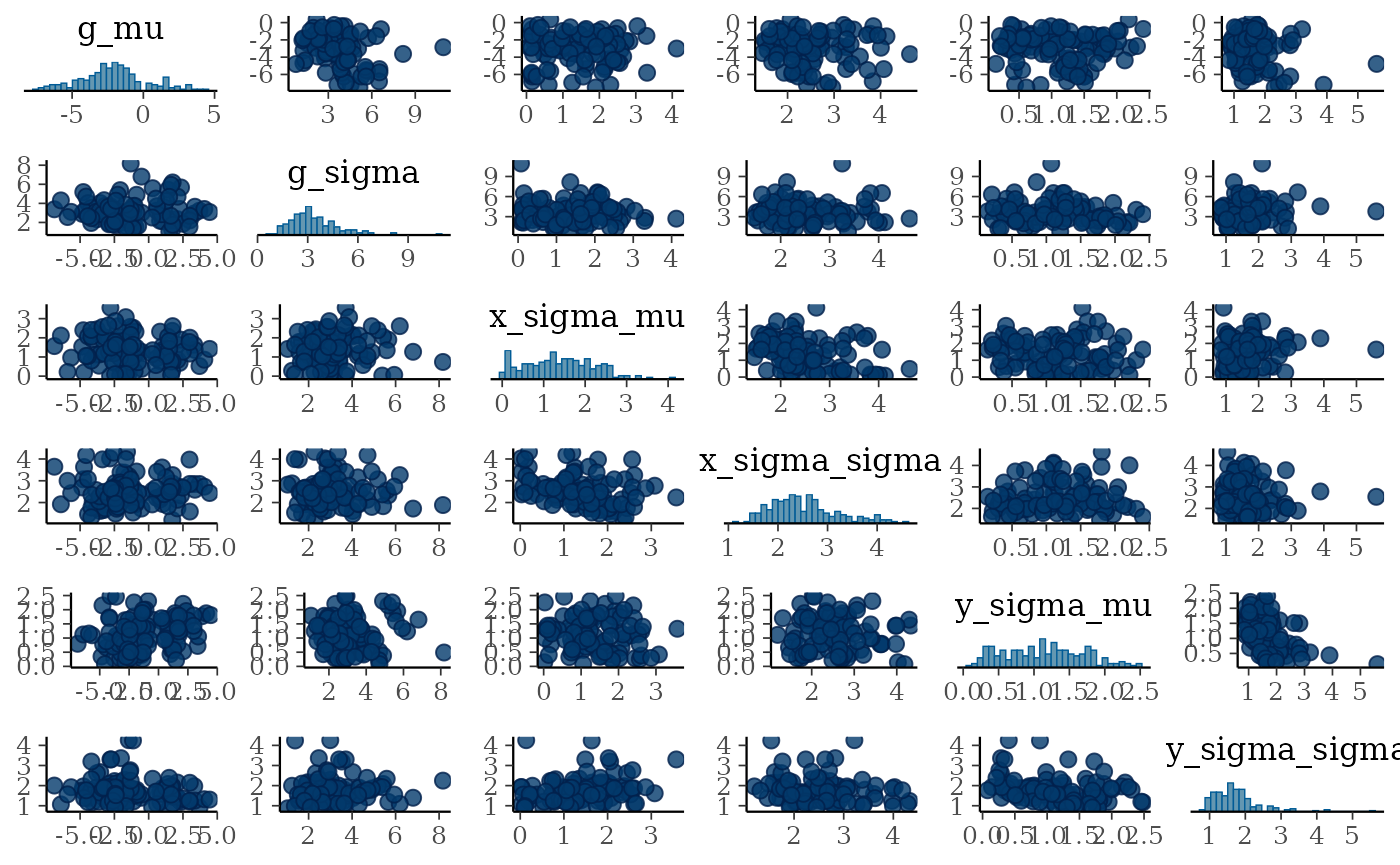

These parameters do not exhibit strong correlations.

For digging deeper into the model, other packages from the Stan development team will be useful. For example, if you have RStan installed, you can use the function rstan::read_stan_csv() to reformat the results and use shinystan.⁴

stanfit <- rstan::read_stan_csv(fit$output_files())
shinystan::launch_shinystan(stanfit)

When applying this model to your data, it is a good idea to browse through these plots. For now, focus on the three main parameters of interest, the average noise at low and high contrast (x_sigma_mu and y_sigma_mu), and the average slope (g_mu). For ease of plotting, convert the posterior samples into a tibble::tibble.

draws <- fit$draws(c("g_mu", "x_sigma_mu","y_sigma_mu")) %>%
  posterior::as_draws_df() %>%
  as_tibble()

Now use tidyverse packages to plot the posteriors. For example, we can look at whether there is evidence that the noise differs across levels of contrast.

draws %>%
  select(-g_mu) %>%
  pivot_longer(cols = contains("sigma"), names_to = "Contrast", values_to = "Noise") %>%
  mutate(
    Contrast = factor(
      Contrast, 
      levels = c("x_sigma_mu", "y_sigma_mu"),
      labels = c("Low", "High"))) %>%
  ggplot(aes(x=Noise, fill=Contrast)) +
  geom_histogram(bins=50, position = position_dodge())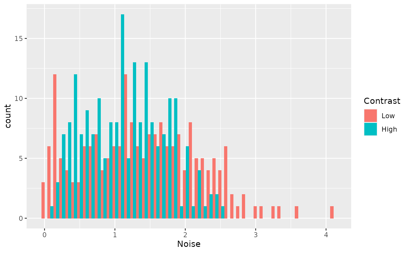

These data provide some evidence that noise increases at high contrast, but the posteriors are not precise enough to be confident.

Finally, what is the average slope?

draws %>%
  select(-contains("sigma"), Slope = "g_mu") %>%
  ggplot(aes(x = Slope)) +
  geom_histogram(bins = 50)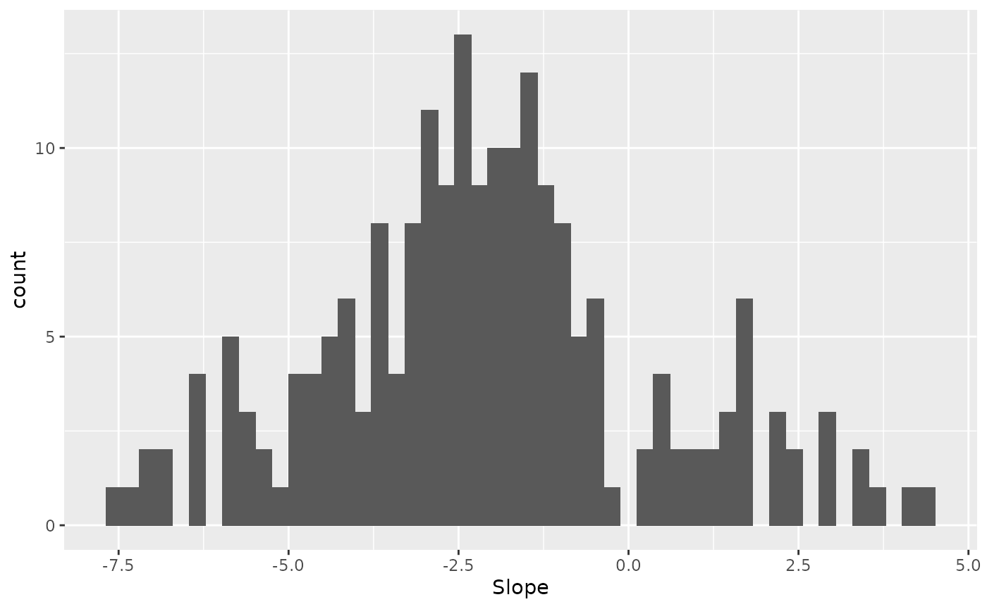

In support of multiplicative gain, the average slope appears to be larger than 1.

Since multiplicative gain but not additive offset predict a slope larger than 1, these data provide evidence that contrast causes multiplicative neuromodulation.

If hierarchical modeling is unfamiliar, see here for a brief introduction.↩︎
The terminology “Deming” refers to this later relaxation.↩︎
The model code is also available on the nmmr repository, here.↩︎
Alternatively, you can use shinystan without installing RStan by instead installing the development version of shinystan. See https://github.com/stan-dev/shinystan/issues/184.↩︎