derivative of gaussian for serial dependence

Cognitive experiments can require participants to complete hundreds of trials, but completing so many trials invariably alters participants’ behavior. Their behavior late in the experiment can depend on their behavior early in the experiment. Although such dependence can be an experimental confound, the dependence itself can provide clues about cognition. One simple kind of dependence occurs through learning; hundreds of trials provides participants ample practice. A more subtle dependence can emerge between sequential trials, an effect called serial dependence. Theoretical interpretations of serial dependence vary, and some of that variability may relate to how the dependence is measured. In this post, I review a statistical method commonly used to analyze serial dependence and discuss one way that method can fail.

I will focus on the analysis of an orientation judgment task, in which participants simply see an oriented bar on each trial, remember the bar’s orientation for a short period, and then report the orientation. Participants’ responses on one trial can depend on the orientation they saw in the previous trial. The dependence follows a Gaussian’s derivative function. Figure 1A shows a Gaussian function with its derivative, and Figure 1B shows the derivative modeling a range of different serial dependence patterns. The derivative captures three key features of the data. First, different changes in orientation between trials result in serial dependencies of different magnitude. The responsiveness of dependence is captured by the width of the derivative. Second, serial dependence can have a different magnitude. The magnitude is captured by the amplitude of the derivative. Finally, responses on the current trial can either be attracted towards or repulsed away from the orientation of the previous trial. The direction of the effect is captured with the sign of the amplitude. The direction of the effect–and the experimental manipulations that change that direction–are often critical to different theoretical interpretations of serial dependence.

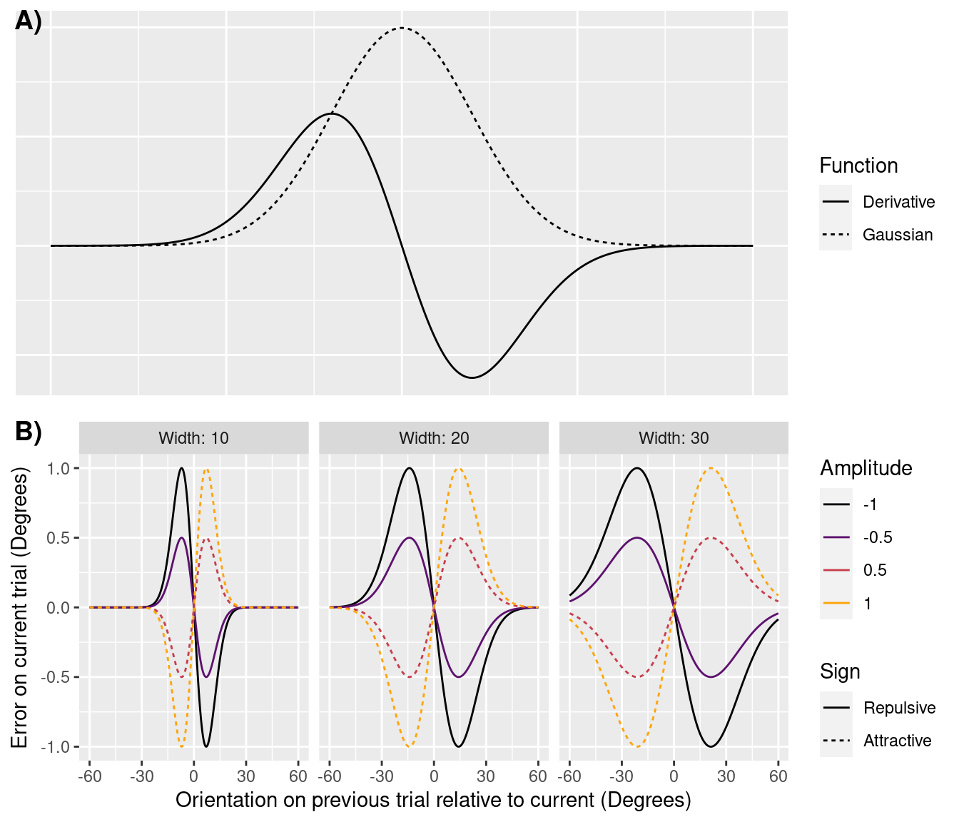
Figure 1: A) A Gaussian function and its derivative. B) The derivative captures how errors on the current trial can depend on how the relationship between the orientation seen in the current and previous trials. Positive values on the horizontal axis signify a clockwise difference and negative values a counterclockwise difference. Likewise, positive errors signify responses on the current trial which were clockwise to the true orientation, and negative errors are counterclockwise. When errors are in the same direction as the difference in orientations, the error is said to be attractive. Otherwise, the error is repulsive. Whether errors are attractive or repulsive is given by the sign of the derivative’s amplitude.

Although the Gaussian’s derivative adequately models the serial dependence between trials with similar orientations (less than 45 degree differences), the derivative fits poorly the dependencies following large changes. When sequential trials have a large orientation difference, the sign of the dependence often changes; small orientation differences can elicit an attractive dependence even while large differences are repulsive. These sign flips are called the peripheral bumps, and they are not captured by the Gaussian’s derivative. If the bumps are large enough, they can interpretations about the sign to of dependencies following small changes can be inverted (Figure 2). Unfortunately, noticing the peripheral bumps can be hard with sparse data. But even with sparse data, the width of the best-fitting derivative can help identify bumps. If the best-fitting derivative is abnormally wide (with peaks larger than approximately 35 degrees), then the derivative is tracking dependencies wider than it should. In that circumstance, it may be best to focus analyses on only the trials with smaller orientation differences.

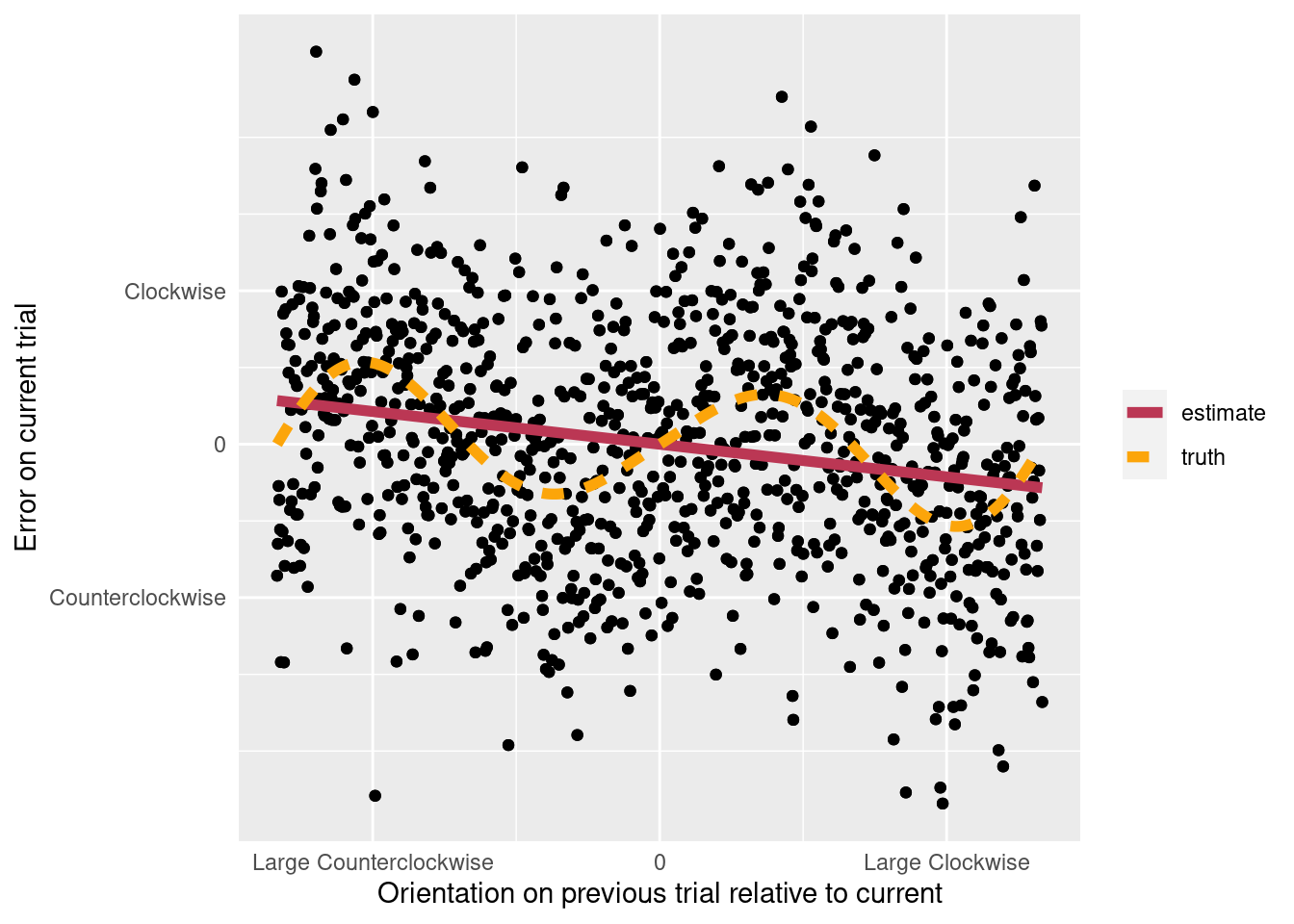
Figure 2: Misfits of the Gaussian’s derivative. The dots give hypothetical data. The data were generated with a function whose average is traced by the dashed line. The data were fit with a derivative of Guassian function, and the best-fitting derivative is shown with a solid line. The derivative does not match the data-generating function.